Does Comsol Automatically Upload Results as You Change

Niggling-known functionality of the Study node is its ability to perform a programmatic sequence of operations, including solving; saving the model to file; and generating and exporting plot groups, results, and images. In this blog post, we take a closer expect at this capability. If y'all use the COMSOL Multiphysics® software, there is a skilful chance you will find this data useful in your modeling work.

Instance: Micromixer Model

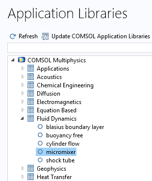
To demonstrate this functionality, nosotros will get-go load the Micromixer tutorial model from the Application Libraries. This model is bachelor in the binder COMSOL Multiphysics > Fluid Dynamics and illustrates fluid flow and mass transport in a laminar static mixer.

The model performs a fluid period simulation using a Laminar Menses interface. In the next step, it shows how to summate the mixing efficiency by ways of a Ship of Diluted Species interface, using the results from the fluid flow simulation as input. The species will be transported downstream based on the fluid velocity.

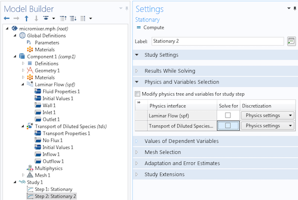
The computation fourth dimension for this model is a few minutes. To simplify the model a fleck so that we tin can run the computation quicker, we won't solve for the species ship. To achieve this, we will make i modification to the Settings window of the 2nd report step, Step 2: Stationary two, past clearing the Send of Diluted Species check box.

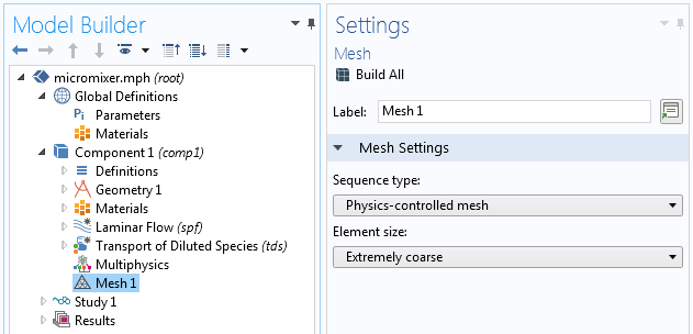
We can make an boosted change to the model in club for it to run faster. Gear up the Sequence type for the mesh to Physics-controlled mesh and the element size to Extremely coarse.

At present, we can compute Study 1 to make certain everything works. The resulting plot shows the velocity magnitude at a few slices along the mixer geometry.

Using Job Sequences to Salvage Information

Here, we will focus our attending on one important part of a job configuration: the Sequence option.

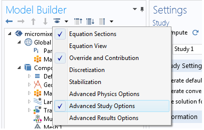
To be able to define a sequence of operations under the Written report node, we enable Advanced Study Options. This is an available menu selection nether the Model Builder toolbar. Click the "center" symbol to see the menu.

Enabling this setting reveals a hidden Task Configurations node in the model tree. This node is something that you don't need to worry most during conventional modeling work. Information technology essentially stores low-level information pertaining to the order in which the solution process should be run. Unremarkably, this is controlled indirectly from the acme level of a study without the need for enabling Advanced Study Options.

Right-click Job Configurations and select Sequence.

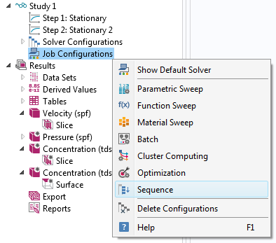
Next, right-click Sequence to see, below the Run option, a diverseness of options that can be added as an ordered sequence of operations performed when running the sequence:

• Job
• Solution
• Other
• Relieve Model to File
• Results

Job refers to another sequence that is to be run from this sequence, while Solution runs a Solution node equally bachelor under the Solver Configurations node, bachelor farther up in the Study tree.

Under Other, you can choose External Class, which calls an external Java® class file. Some other option, Geometry, builds the Geometry node. This can be used, for instance, in combination with a parametric sweep to generate a sequence of MPH-files with different geometry parameters. The Mesh option builds the Mesh node.

Relieve Model to File saves the solved model to an MPH-file.

Under the Results option, y'all can choose Plot Group to run all or a selected set of plot groups. This is useful to automate the generation of plot groups after solving. Yous also don't take to manually click through all of the plot groups to generate the corresponding visualizations. The Derived Value choice is there for legacy reasons and we recommend that you lot use the Evaluate Derived Values option, which will evaluate nodes nether Results > Derived Values. The option Export to File runs any node for data export nether the Export node.

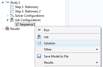
Let's at present create a simple sequence. Correct-click the Sequence node and select Solution.

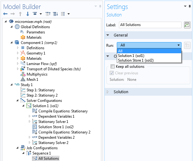
The default option for a Solution node in a sequence is to run all solution nodes. The Run pick in the Full general section lets yous specify which Solution information structures should exist computed. The Solution information structures are available every bit child nodes, together with other nodes, under Solver configurations. They tin can exist recognized past their brusque proper noun written inside parentheses, such equally (sol1) and (sol2). The solution data structures are low-level representations of the solutions.

In this example, you tin keep the default All for the Solution data structures.

Nosotros would like to save the file when the solver is finished. Right-click the Sequence node and select Save Model to File.

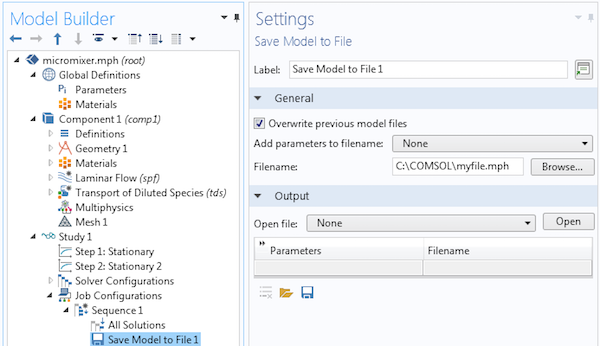
In the Settings window, you can run into a number of options that are related to the capability of saving a series of MPH-files with parameters added at the stop of the file name. This is very useful for parametric sweeps such as batch sweeps. However, nosotros will not need to exercise this in such a simple case, so we change the pick Add parameters to filename to None. At this phase, we also need to give a file name to a location where nosotros have permission to write. In this example, the file proper name and path is C:\COMSOL\myfile.mph.

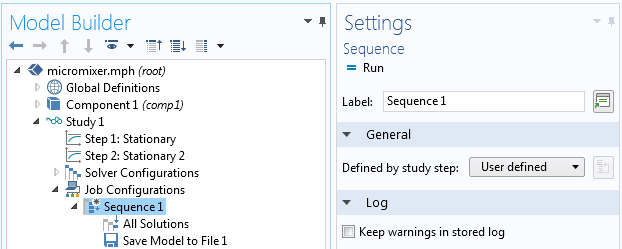
To run these operations, select the Sequence node and click Run.

Writing Data to File After Solving in COMSOL Multiphysics®

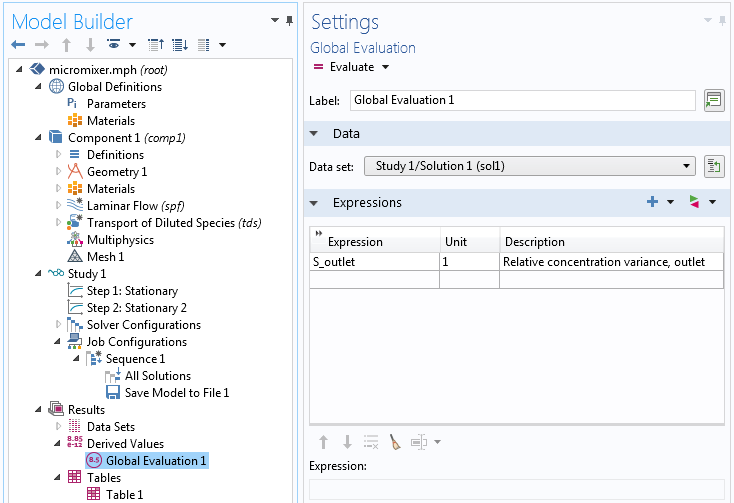
The library model that nosotros started from already has one defined derived value. You lot can come across this nether Results > Derived Values > Global Evaluation. The variable is called S_outlet and is the relative concentration variance at the outlet. It is defined as a variable nether Component > Definitions > Variables.

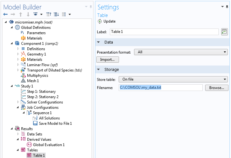
The value of S_outlet is sent to Table 1. We can choose to store this value on file by changing a setting in the Settings window of Table 1. Alter Store table to On file and type a file name; for example, C:\COMSOL\my_data.txt.

Now, add together an Evaluate Derived Values functioning to the sequence.

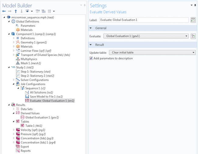
In the General section, yous tin change the Evaluate setting to Global Evaluation 1. However, in this simple instance model, you lot can omit this step. Note that the name of the node in the model tree changes to Evaluate: Global Evaluation 1.

Y'all can now run the sequence again. However, for this concluding step to make sense, you demand to enable the Transport of Diluted Species interface in the Settings window for Step ii: Stationary 2.

Running Task Sequences from the Command Line

If you want to run a chore sequence from the command line in the Windows® or Linux® operating systems, or macOS, you cannot utilise the method shown above, but instead you demand to add together a parametric sweep with a dummy parameter. However, if you were already running a parametric sweep, so all you need to know is that a parametric sweep is just a special type of job sequence and so follow the instructions above, merely with a Job Configurations>Parametric Sweep node replacing a Job Configurations>Sequence node.

The reason for this is historical and reflects the evolution of the Report node functionality over time. The operating system command interface doesn't permit y'all run any part of a Study node that is non controlled at the top level of the Study node. You can only specify which report to run, for example, in the Linux® operating system:

comsol batch -inputfile mymodel.mph -report std1

for Written report 1 with tag std1.

You cannot run a sequence in this way, since the peak-level written report step is unaware of your edits nether the Chore Configuration node. To make the study stride at the meridian of the Study node tree "enlightened" of your edits under the Job Configurations node, the easiest way is to add a parametric sweep with an arbitrary parameter defined under Global Definitions > Parameters; say, dummy with value 1. Sweeping over this parameter then adds the extra overhead needed to get a handle on the Task Configuration node from the acme level of the Written report node. Then, you can outcome a command-line batch command to run information technology.

This is how the corresponding "dummy" sweep will look:

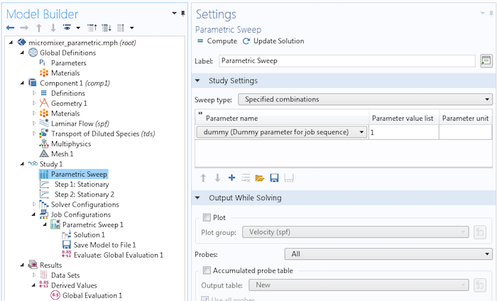
The following figure shows the corresponding sweep over one parameter value for the dummy parameter.

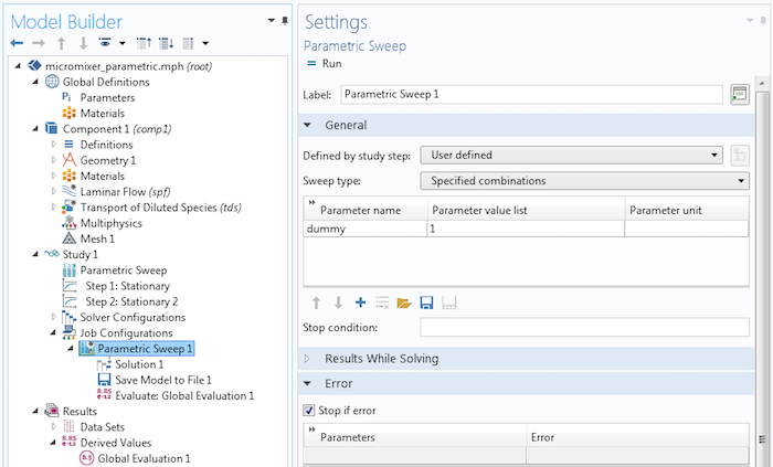
Now, knowing that the Parametric Sweep 1 node is simply a special type of Sequence node, the kid nodes Solution 1, Save Model to File i, and Evaluate: Global Evaluation 1 are just as they are in the example to a higher place using Sequence.

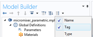
Enable the brandish of model tree tags past selecting Tag from the Model Tree Node Text menu, available in the Model Builder toolbar.

The report tag std1 is now visible in the model tree:

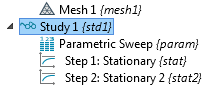
The Linux® command shown earlier will now run the sequence of operations that solves, saves the model to file, and finally evaluates the Global Evaluation node. Note that if you but accept one Study node in your model, then you tin can skip the input argument written report std1.

Annotation that if you lot already have a parametric sweep in your model, these can be of two types loosely referred to as "inner sweep" and "outer sweep". The sweep in the example in a higher place using the dummy parameter is an "outer sweep". The Report node will autodetect which type of sweep to employ for all-time performance, but you tin can take control manually, if needed. In order to use a job sequence from the control line, your sweep needs to be an "outer sweep".

More than or less all types of sweeps can exist changed from being an inner sweep to an outer sweep, but not the other style around. Inner sweeps can be faster, since they will use some of the underlying structure of the computation to speed things up. However, not all types of sweeps can be inner sweeps. For example, a sweep over a geometry parameter always needs to be an outer sweep; again, this is handled automatically by the solver. To make certain the parameter sweep is an outer sweep, change the Employ parametric solver to Off in the Parametric Sweep settings, then perform a Testify default solver operation and keep from there.

Summary

Job sequences tin can be used to automate a number of common tasks after solving a model. In this blog post, nosotros have seen examples of:

• Saving the model to file as an MPH-file after solving
• Exporting Derived Values to file automatically subsequently solving

At that place are other tasks that use job sequences that y'all tin can endeavour on your own, including:

• Regenerating all plots afterward solving
• Exporting plot information to file
• Exporting image information to file

Nosotros hope yous find that job sequences are a useful feature for your everyday modeling work!

Oracle and Java are registered trademarks of Oracle and/or its affiliates. Microsoft and Windows are either registered trademarks or trademarks of Microsoft Corporation in the United States and/or other countries. Linux is a registered trademark of Linus Torvalds in the U.S. and other countries. macOS is a trademark of Apple tree Inc., registered in the U.South. and other countries.

durhamallons1966.blogspot.com

Source: https://www.comsol.com/blogs/how-to-use-job-sequences-to-save-data-after-solving-your-model/